1.
 Introduction
This chapter has the following sections:
1.1. Function and parameter optimization
1.2.
Problem Formulation
1.2.1.Design variables
1.2.2.Constraints
1.2.3.Objective function
1.4.
Exercises
1.5. References
![]()
1.1.
Function and parameter optimization 
Structural Optimization deals with the efficient design of structures. Efficiency implies minimum cost or minimum weight while satisfying a variety of strength and stiffness requirements. Until the early 1980s, structural optimization was mostly the domain of researchers in universities or government laboratories. Then industry started making use of the techniques developed by researchers, and today these techniques are commonly applied in a large spectrum of industries, ranging from aerospace and civil to automotive engineering.
The origins of the optimization theory are formed as a study in Mathematics. Early applications used the calculus of variations to seek functions that will minimize or maximize a functional. A classical example of this approach was the so-called brachistochrone problem, of finding the functional form of a path that minimizes the time for a particle to roll from point A to point B in a vertical plane (Fox, 1987, p.24). Early applications of structural optimization also used the calculus of variations and employed the differential equations that govern the behavior of the structure. The structural response (e.g., displacements or stresses) was defined as functions over a continuum, and structural optimization sought functions describing the distribution of the optimal structural properties. A typical application was the design of a beam for minimum weight, with the optimum defined in terms of the variation of moment of inertia over the length of the beam (e.g., Barnett, 1961)
In contrast, for most industrial applications, structural optimization uses analysis methods that discretize the structural domain, notably finite element methods. The properties of the design are described by scalars associated with the form of discretization rather than by functions. For example, a beam structure may have design variables that define the moment of inertia of each beam element that make up the structure. The element is assumed to have a constant cross section along its length. Figure 1.1.1 contrasts the function optimization and parameter optimization of the moment of inertia of the beam.
The mathematical discipline that deals with parameter optimization is called mathematical programming. The bulk of this courseware deals with mathematical programming techniques and their application to structural optimization problems defined by discretized models. In particular, it is often implicitly assumed that the structure is modeled by finite elements.
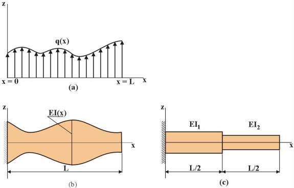
Figure 1.1.1
Beam example: (a) Loading; (b) Function optimization for EI(x); (c) Parameter
optimization for EI1 and EI2.
1.2.
Problem
Formulation 
We formulate a structural optimization problem as a mathematical optimization problem in a specific mathematical form. The problem is to minimize or maximize a function f of n variables, xi, i=1, 2,…, n. The variables are components of a vector denoted in boldface lowercase letters,
 . (1.2.1)
A general mathematical optimization problem also includes a set of functions that are posed as constraints. A more in-depth discussion of the physical significance of the constraints and the function to be minimized will be provided in the following sections. It will suffice to present the mathematical form here as,
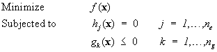 (1.2.2)
where ne is the number of constraint functions that are posed as strict equalities and ng is the number of inequality constraints. Properly casting a structural design optimization problem into this mathematical form is one of the crucial steps of a design optimization effort and will be described in the following.
1.2.1.
Design Variables 

The design of the structure is often a matter of sizing dimensions, such as thicknesses of plate and shell segments or cross-sectional areas of bars. In some problems, the design involves selecting shapes, such as the optimal shape of a hole. The dimensions and the shapes are usually defined in terms of a number of scalar parameters called design variables. In this courseware, we denote the design variables by their mathematical representation, which are the components of a vector x, with the exception that the expanded form of the vector is shown with regular parentheses rather than curly ones and the transpose sign is dropped for convenience,
![]() (1.2.3)
(1.2.3)
This
vector represent a point in the design
space ![]() spanned by the design
variables, that is x Î Rn. In the sequel, we call this vector and the
associated structure a design.
spanned by the design
variables, that is x Î Rn. In the sequel, we call this vector and the
associated structure a design.
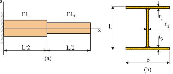
Figure 1.2.1 Cantilevered I-beam with two segments. (a)
overall view; (b) cross-sectional shape
In the beam example of Figure 1.2.1, the moments of inertia ![]() and
and ![]() of the two segments
can be two design variables. After the
optimization is concluded, the designer will need to design the details of the
cross section, or find a commercially available cross section with a close
match to the optimal moments of inertia.
This approach of having a single design variable per beam segment is
common when the design is governed mostly by stiffness consideration. When stresses in the beam cross-section are
an important design consideration, then the details of the cross section may be
included as design variables.
of the two segments
can be two design variables. After the
optimization is concluded, the designer will need to design the details of the
cross section, or find a commercially available cross section with a close
match to the optimal moments of inertia.
This approach of having a single design variable per beam segment is
common when the design is governed mostly by stiffness consideration. When stresses in the beam cross-section are
an important design consideration, then the details of the cross section may be
included as design variables.
If the beam is constructed by welding steel plates to form the
I-section, as shown in Figure
1.2.1(b), it is natural to choose the plate thicknesses ![]() as design variables,
for a total of six design variables (three per beam segment). The breadth
as design variables,
for a total of six design variables (three per beam segment). The breadth ![]() and height
and height ![]() of each cross section
can be additional design variables (for a total of 10) or may be fixed as
pre-assigned parameters. It is possible
to reduce the number of design variables by assuming both flange thicknesses to
be equal, i.e.,
of each cross section
can be additional design variables (for a total of 10) or may be fixed as
pre-assigned parameters. It is possible
to reduce the number of design variables by assuming both flange thicknesses to
be equal, i.e., ![]() =
= ![]() for each segment,
reducing the total number back to eight.
The numerical solution of an optimization problem becomes more difficult
when the number of design variables is increased. On the other hand, if the optimum can be successfully found, the
value of an objective function usually improves with additional design
variables.
for each segment,
reducing the total number back to eight.
The numerical solution of an optimization problem becomes more difficult
when the number of design variables is increased. On the other hand, if the optimum can be successfully found, the
value of an objective function usually improves with additional design
variables.
Another illustrative example, a nine-bar truss under
two vertical loads, is shown in Figure
1.2.2.
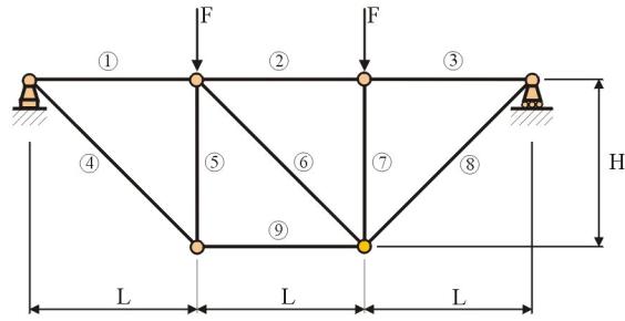
Figure 1.2.2:
Nine bar truss
Again, several choices for design variables are
possible. Perhaps the most common
choice consists of member areas ![]() as design variables,
with the dimensions H and L fixed. The design variable vector is then
as design variables,
with the dimensions H and L fixed. The design variable vector is then
If the height and the span can also be changed, the
design variable vector expands to
One approach to reduce the number of design variables in Eq. (1.2.5) is
to form groups of bars, each having the same member area. For example, we can set all the horizonal
bars to have one design variable,![]() ; the two vertical bars to have another,
; the two vertical bars to have another,![]() and the three slanted bars to have the third,
and the three slanted bars to have the third,![]() . Then the formulation with cross-sectional design variables,
Eq. (1.2.4) has only
three components, and the formulation including the geometrical dimensions only
five.
. Then the formulation with cross-sectional design variables,
Eq. (1.2.4) has only
three components, and the formulation including the geometrical dimensions only
five.
All the design
variables described above assume values that are positive, because it does not
make any sense for a physical dimension of a structure to be a negative
number. In some cases design variables
that have negative values must be used.
[Rafi,
how do you feel about explaining how to represent (-)ve design variables
for linear programming algorithms that work with only (+)ve variables in here?
I think that this should wait until that chapter.
Even then it should appear only in a web version that requires a click in order
to see it.]
It is important for
the design variables to describe fully the design configuration. However, it is also important that the will
be independent. It is possible inadvertently to choose redundant
variables. For example, for the design
of a tubular member, one may choose the inner and outer radii, ri and ro respectively, and the wall thickness, t, as design variables. Clearly, one needs only two of the three
variables to fully describe the cross-sectional geometry. If it is convenient to use all three
variables in the design formulation, the geometric relation between them, ro = ri
+ t must be maintained during the design process
as a constraint. However, more design
variables and more constraints make the problem more difficult to solve.
Therefore, whenever possible, it is better to avoid using redundant variables
and the associated equality constraints.
Design
variables may take continuous or discrete values. Continuous design variables have a range of
variation, and they can take any value in that range. For example, the cross-sectional areas of the nine-bar truss in
the example above would be mostly used as continuous design variables in some
range of minimum and maximum cross-sectional areas. Discrete design variables, on the other hand, usually take only a
finite number of permissible values.
For example, if the bars for the truss must be made from commercially
available cross sections, then only a finite number of cross-sectional areas
are possible. Material design variables
that decide what material is used are typically assigned integer values
corresponding to a list of materials.
For example, a value of one may correspond to aluminum, a value of two
to steel, etc.
We
often disregard the discrete nature of the design variables. Once we obtain the optimum design, we adjust
the values of the design variables to the nearest available discrete value. This approach is popular because an
optimization problem with discrete design variables is usually much more
difficult to solve than a similar problem with continuous design
variables. Rounding off the design to
the closest discrete solution may work well when the available values of the
design variables are closely spaced.
Then changing the value of a design variable to the nearest discrete
value does not change much the response of the structure. In some cases, the discrete values of the
design variables are spaced so far apart that we must solve the problem by
using discrete variables. For this we
employ a branch of optimization theory called integer programming. In
this courseware, design variables are continuous unless otherwise stated.
Finite
element models usually require elements that are small compared to the length
scale of the variation in structural properties. Because design variables often
define that length scale, we have to be careful not to have more design
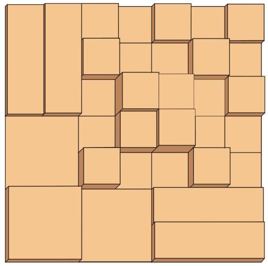
variables than the finite element model can support. For example, the plate shown in Figure
1.2.3 was analyzed (Prasad
and Haftka, 1979) by a fixed ![]() finite element mesh,
with most design variables specifying the thickness of the individual
elements. While the
finite element mesh,
with most design variables specifying the thickness of the individual
elements. While the ![]() model was adequate
for the initial design, which had a uniform thickness, it was not adequate for
the final design shown in the figure.
model was adequate
for the initial design, which had a uniform thickness, it was not adequate for
the final design shown in the figure.
Figure 1.2.3: Plate
thickness optimization.
A
similar problem may surface when the coordinates of nodes of the finite element
model serve as design variables. For
example, the shape of the hole in the plate shown in Figure 1.2.4 was optimized (Braibant
et al., 1983Ref_Barnett61)
to reduce the stress concentration near the hole. The coordinates of all
the boundary nodes of the hole served as design variables. Again, the finite element mesh depicted in
the figure was adequate for the analysis of the initial square hole. The final shape shown in Figure
1.2.4 clearly does not represent the optimal
shape. The optimization procedure took
advantage of the large number of design variables to reduce the objective
function by increasing the error in the computation rather than by reducing the
true stress concentration. In general,
the distribution of design variables should be much coarser than the
distribution of finite elements. Only
in skeletal structures, where finite elements often correspond to physical
structural elements, a similar distribution for elements and design variables
may be natural.
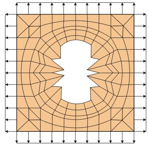
Figure 1.2.4: Hole shape optimization
1.2.2. Constraints 
The
design of a structure is normally subject to requirements or limitations. Typical requirements specify that the
structure must be safe, for example, that stresses do not exceed material
limits. Stress limits are also often
specified by standards and design codes or by customers. Manufacturing requirements may also
constrain design freedom, for example, limiting the number of different
sections that we can use. In
mathematical optimization, equality and inequality constraints introduce these requirements. In this courseware, inequality
constraints are expressed as
![]() (1.2.6)
(1.2.6)
The
constraint function gj(x) may in represent any
economic, physical or technical quantity that depends on at least one design
variable. In structural optimization,
typical constraints are functions of stresses, displacements, buckling loads,
fatigue life, and natural vibration frequencies. It is possible to reverse the sense of an inequality of the
opposite type
![]() (1.2.7)
(1.2.7)
to the standard form
used in this courseware by multiplying it by ![]() . Unfortunately,
inequalities of both senses are widely used in the literature, and the choice
affects the sign convention in many of the results obtained in this courseware.
. Unfortunately,
inequalities of both senses are widely used in the literature, and the choice
affects the sign convention in many of the results obtained in this courseware.
When
inequality constraints simply specify upper and lower limits on the design
variables they are called side
constraints and often treated separately from other constraints. They are expressed as
![]() (1.2.8)
(1.2.8)
where ![]() is the given lower
limit and
is the given lower
limit and ![]() the given upper limit
for design variable
the given upper limit
for design variable ![]() .
.
Equality
constraints are not common in structural optimization. They often appear in special formulations
where the analysis and design are integrated into a single problem. In such formulations, the structural
response (e.g., displacement) components are used as additional design
variables, and the equations of equilibrium are imposed as equality constraints. In a more standard formulation, equality
constraints appear when a response quantity, such as a frequency, must take a
specified value.
Equality constraints are expressed
here as,
The number of
independent equality constraints must be naturally smaller than the number of
design variables. Otherwise, there is
no design freedom and so no optimization problem to solve. Each equality constraint in Eq. ![]() (1.2.9) represents a hyper-surface on which the design
should lie. Equality constraints
restrict design freedom more severely than inequality constraints and are more
difficult to handle numerically. It is
desirable, whenever possible, to avoid equality constraints by reformulating
the problem.
(1.2.9) represents a hyper-surface on which the design
should lie. Equality constraints
restrict design freedom more severely than inequality constraints and are more
difficult to handle numerically. It is
desirable, whenever possible, to avoid equality constraints by reformulating
the problem.
A
design that satisfies all the constraints is called a feasible design or feasible
solution. The part of the design
space where all constraints are satisfied is called feasible region or feasible
set. In the following, ![]() is used for the
feasible set, which is defined as follows
is used for the
feasible set, which is defined as follows
![]() (1.2.10)
(1.2.10)
A feasible point x
Î W can satisfy an
inequality constraint as an equality or with a margin. In the former case, the constraint gj(x) = 0 is called active.
In the latter case gj(x)
< 0 , and the constraint is said to be passive
or inactive. If a design x
violates at least one constraint, gj(x)
> 0 , then this design is called infeasible. In most numerical optimization software, the
boundary between the feasible domain and infeasible domain is not so
sharp. That is, a constraint is
considered satisfied even if it is violated by a small amount. Similarly, a constraint is considered active
even if it is satisfied by a small margin.
These tolerances cater to small errors in evaluating constraints, and
often improve the performance of the optimization solution procedure.
1.2.3. Objective function 
In
order to find the best feasible design, we must have a criterion, such as cost,
weight, stiffness, or strength that ranks designs. This criterion as a function of design variables is called objective function. If the objective function is better when
large (e.g., stiffness), then the optimization problem is a maximization
problem. If the objective function is
better when small (e.g., weight) than it is a minimization problem. The objective is denoted here by f(x), with f : Rn ® R.
Other terms, such as cost function, merit function or performance index
have also been used for objective function.
In this courseware, all problems are formulated as minimization but this
does not exclude the consideration of maximization problems. Since
![]() , (1.2.11)
, (1.2.11)
any maximization problem
may be easily converted into a minimization problem.
For
many practical problems, however, the choice of just one objective function to
rank designs is difficult. Instead,
several competing criteria should be considered simultaneously. In structural optimization, cost, weight,
maximum stresses, displacements, vibration frequencies, buckling or limit
loads, and the probability of failure are typical criteria. It is possible to have several objective functions
using multicriterion optimization. This topic is treated in detail in Chapter
xx, and in the rest of the courseware, a single objective function is
assumed. Material volume or structural
weight is the most common objective function found in the literature of
structural optimization. It is a simple
and often linear function of design variables.
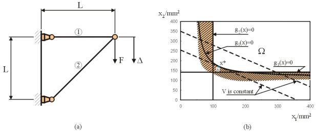
As
an introductory example, consider a two-bar truss shown in Figure
1.2.5 (a). The structure
is loaded by vertical force F = 20 kN at the free node. Minimize the material volume, V, of the
truss when the allowable stresses in the bars are s u = 200 N/mm2
in tension and s
l = 200 N/mm2 in compression. In
addition, the vertical displacement of the loaded node is limited to be below Du = 2.5
mm. Cross-sectional areas of both bars
are used as design variables. The truss
is made of steel with a modulus of elasticity E = 2.0´105 N/mm2, and
the length L = 1000 mm. Ignore possible
buckling of the compression bar.
Solution:
In this statically determinate case, explicit
expressions for the stresses and the vertical displacement are easily
obtained. Denoting the member area of
bar 1 by x1 and of bar 2
by x2, the following
optimization problem is obtained,
Here V is the
objective function, which represents the material volume of the truss. It is a linear function of the design
variables and is minimized subject to displacement constraint (1.2.13) as well as stress constraints (1.2.14) and (1.2.15). In this simple case, an explicit problem
formulation without equality constraints can be obtained. Constraint functions defined in the standard
form ![]() (1.2.6) are
(1.2.6) are

![]() (1.2.18)
(1.2.18)
where
x
= (x1, x2) is the design variable
vector. With only two design variables,
we can solve the problem graphically.
This is shown in Figure 1.2.5 (b) where the feasible set W has been
depicted by drawing curves gj
= 0, j = 1, 2, 3 in the design plane R2
and checking that all constraints (1.2.12-14) are satisfied simultaneously. The feasible set W is obtained as
an intersection of those three regions, which correspond to cases g1 £ 0, g2 £ 0 and g3 £ 0. It is the unshaded region in the top right
part of the figure.
Figure 1.2.5:
Two bar truss.
In
addition, two lines of constant objective function, called objective function
contours, which are straight lines according to ![]() (1.2.12) are depicted in Figure
1.2.5 (b). Along
these lines, the material volume has a constant value. The lower contour, which just touches the
feasible set, corresponds to the optimum value Vmin = 360,000 mm2. The optimal solution is achieved at point A
where x1* = 120 mm2 and x2*
= 170 mm2. In this problem,
only displacement constraint
(1.2.12) are depicted in Figure
1.2.5 (b). Along
these lines, the material volume has a constant value. The lower contour, which just touches the
feasible set, corresponds to the optimum value Vmin = 360,000 mm2. The optimal solution is achieved at point A
where x1* = 120 mm2 and x2*
= 170 mm2. In this problem,
only displacement constraint
 (1.2.16)
is
active, i.e., g1(x*) = 0.
1.3.
Graphical Optimization 
The mathematical formulation presented in the previous section can best be solved using numerical methods, which will be described in some details in the following chapters. However, when the design problem can be formulated in terms of only two design variables, graphical methods can be used to solve the problem as demonstrated by Example 1.2.1. Graphical methods are not the most efficient methods of solution, because they require a large number of evaluations of the objective functions and constraints, but they help designers gain a valuable understanding of the nature of the design space. Moreover, because visualizing the design space is a powerful tool for understanding the trade-offs associated with a design problem, graphical methods are often used even when the number of design variables exceeds two. In that case, we look at special forms or reformulations of the design problem. For example, all of the design variables may be fixed except two that are allowed to vary.
There is a variety of media for performing graphical solutions of an optimization problem, the most traditional being paper and manual drawing tools. However, most modern engineering software, such as Mathematica and Matlab, provide functions that allow convenient graphical representation of an optimization problem.
The first step in solving an optimization problem graphically is to visualize the dependence of the objective function on the two design variables. The standard approach that mapmakers have used for generations is often used for this purpose. Contour lines as in Figure 1.2.5(b) representing lines with equal value of the function are drawn. In weather maps, these are usually isotherms (lines of equal temperature) or isobars (lines of equal atmospheric pressures). For graphical optimization, these lines are called function contours. Function contours can be created in many different ways. We can take the expression for the function, set it equal to a constant, and solve for one of the variables in terms of the other one. This will give us an equation for one of the curves. Repeating the process of other values of the constant completes the contour lines. Alternatively, we can cover the region of interest with a dense grid of points, calculate the function value at each one of the points, and find by interpolation where the function has a desired value to draw the line associated with that value. Again, the process is repeated for other values of the function to complete the contour lines.
Once the contour lines are drawn, regions where the objective function is high are denoted in different shadings or colors than regions where the objective function is low. In a weather map, for example, high temperatures are denoted in red and low temperatures in blue. The software packages mentioned earlier can draw function contours automatically and include numerous options to change the appearance of the contour map.
If there are
no constraints other than side constraints, the plane region defined by the
ranges of the design variables used in the graphical representation represents
all possible combinations of the two design variables. This region is typically referred to as the
design space. For constrained problems,
parts of the design space are unacceptable.
Therefore, the next step in graphical solution is to draw a boundary
line for each of the constraint functions (both inequality or equality
constraint) superimposed over the objective function contour plot. Unlike the objective function, which we do
not know its value at optimum, the value of the constraint function along the
boundary line is zero for a problem specified in the standard form of Eqs. ![]() (1.2.6) or
(1.2.6) or ![]() (1.2.9). The
difference between the equality and inequality constraints is in the
interpretation of the design space.
Constraints divide the design space into feasible and infeasible
parts. A section of the design space
that violates a constraint function is termed infeasible region. Because the equality constraint requires the
value of the constraint function to be identical to zero, any other contour
line, hi ≠ 0,
which is a line on either side of the hi = 0 line is in the infeasible region. Hence, the only feasible portion of the
two-dimensional space is the line segment corresponding to an equality
constraint line. In the case of
inequality constraints, only one side of the gi = 0 line, which correspond to the constraint function
values greater than zero (the positive values) is unacceptable. To graphically indicate the region of the
design space that is infeasible, the convention is to draw hatch lines on the
side of the constraint that is infeasible.
(1.2.9). The
difference between the equality and inequality constraints is in the
interpretation of the design space.
Constraints divide the design space into feasible and infeasible
parts. A section of the design space
that violates a constraint function is termed infeasible region. Because the equality constraint requires the
value of the constraint function to be identical to zero, any other contour
line, hi ≠ 0,
which is a line on either side of the hi = 0 line is in the infeasible region. Hence, the only feasible portion of the
two-dimensional space is the line segment corresponding to an equality
constraint line. In the case of
inequality constraints, only one side of the gi = 0 line, which correspond to the constraint function
values greater than zero (the positive values) is unacceptable. To graphically indicate the region of the
design space that is infeasible, the convention is to draw hatch lines on the
side of the constraint that is infeasible.
Once the feasible and infeasible portions of the design space are identified, the final step is to identify the optimal solution by inspection. Naturally, if we are trying to minimize the objective function, we will move in the feasible domain to a point that has the smallest objective function value. This can be accomplished by moving to the contour line with the lowest value of the objective function in the feasible domain. If that lowest contour line is entirely in the feasible domain, the minimum lies inside the closed domain formed by that contour line and is away from the constraint boundaries. In this case, none of the inequality constraints dictates the location of the optimal solution; hence, they are referred to as being inactive constraints. This situation is rarely encountered in structural optimization because most problems have important constraints that are active at the optimum.
If the lowest contour line intersects the boundary of one or more inequality constraints, then some or all of these constraints dictate the location of the optimal solution and are called active constraints. The active constraints are identically satisfied at the optimum, gi = 0.
If the determination of the optimal solution via inspection is difficult because of graphical resolution, then there are two possible remedies. The first one is to zoom in on the region around the place of expected optimum by redefining the range of the two design variables and drawing the objective function contours with finer increments. This can be done repeatedly until a desired level of resolution in the design variables is achieved.
The second remedy involves mathematical manipulation of the objective function and the active constraint equations. If there are two active constraints, then it may be possible to solve the two equations and determine the exact value of the optimal design variables. If there are more then two active constraints, then any two of the constraints may be picked up for solution, and the solution should satisfy the other active constraints.
In the case of a single active constraint, a solution involving a two-step process is possible when the objective function and constraints are differentiable. First, since the constraint is satisfied exactly, the active constraint equation may be solved for one of the design variables in terms of the second one. Substituting the solution of the constraint equation into the objective function reduces it to a single variable. Finding the optimum value of a function with a single variable can then be accomplished by equating its derivative with respect to the variable to zero.
There is one more possibility in case of a single active constraint. If, upon substitution of the solution of the constraint equation for one of the variables in terms of the other one reduces the objective function to a constant value (rather then reducing it to a function of the other variable), then the objective function contours are parallel to the constraint boundaries. This implies that all the points along the constraint boundary are optimal solutions.
Finally, if the optimum is unconstrained and the objective function is differentiable, then its exact location may be found by setting the derivatives of the objective function to zero.
We will use the following example of the design of a soft-drink-can to discuss some of the basic concepts associated with graphical optimization described above.
Example 1.3.2
A soft-drink company has a new drink that they
plan to market, and through preliminary research it was found that the cost C
to produce and distribute a cylindrical can for the drink is approximately
where Vo is the volume in
fluid ounces, and S is the surface area of the can in square
inches. They also determined that they
can sell the drink in cans ranging from 5 to 15 ounces, and then the price P
in cents that can be charged for a can is estimated as
Based on their past
experience they will consider only a can with diameter D between 1.5 and
3.5 inches, and their market research has shown that soft-drink cans have to
have an aspect ratio of at least 2.0 to be easy to drink from. That is, the height H of the can has
to be at least twice the diameter.
The objective of the
company is to design the can so as to maximize their profit from the sales of
the soft drink. Two measures of profit
are considered. One is the profit per
can, and the other is the profit per ounce of the drink. The first measure is more useful if we
assume that consumers will buy a fixed number of cans, and the other if we
expect consumers to buy a fixed volume of drink.
Solution:
We first consider the
three elements that go into formulating this design example as a mathematical
optimization problem (see Section SecOptForm). First, the design variables that are needed
to specify the shape of the can. In
this case, the diameter D and the height H are natural design
variables. However, we could use the
radius of the can instead of the diameter, and conceivably even use the volume
and surface area as design variables and calculate from them the diameter and
aspect ratio of the can.
Next we consider the
two objective functions, the profit per can and the profit per ounce, as
functions of the design variables. We start by expressing the volume and the
surface area in terms of the diameter and the height of the can
where the 1.8 factor
is used to convert from cubic inches to fluid ounces. The first objective function, profit per can pc,
may be then written as
![]() .
.
We can get an explicit expression for pc
in terms of the design variables by substituting P
and C into this
equation to obtain
However, it is not
necessary to obtain such explicit expressions. Instead the collection of
equations for substituting P and C constitutes
a procedure for calculating pc as a function of D and H
that we can denote as pc (D, H). In fact, if we write a computer program to evaluate pc,
using the individual expressions is more convenient, more error free, and
simpler to understand for somebody reading the program than using the implicit
expression given above.
The second objective
function, the profit per ounce, can be obtained by dividing pc by
the volume.
We can again
substitute the expression for pc and the expression for Vo to obtain an explicit expression
for pc (D,H). However, this is not needed.
Finally, let us
consider the expressions for the constraints in this problem. The first set consists side constraints that
are the lower bound and an upper bound for the diameter
![]() .
.
Next is the aspect-ratio constraint,
![]() .
.
Finally we have the constraints on the volume,
![]()
By substituting the expression for the volume, we can rewrite this
expression as
Both the side
constraints and the aspect ratio constraint are inequality constraints.
We can now formulate the soft-drink-can example
in standard format using normalized constraints. Using the profit per can as objective function, and changing the
sign to transform the problem to minimization, we get
![]()
The aspect ratio
constraint and the volume bound constraints are normalized as
To help in converting
the formulation to the standard format, we will write the entire problem with D
replaced by x1, H replaced by x2,
and the objective function denoted as f. Then we get
![]()
 (1.3.3)
The first step in
solving an optimization problem graphically is to visualize the dependence of
the objective function on the 2 design variables. Regions where the objective
function is high are denoted in different shadings or different colors as
compared to regions where the objective function is low.
The following figure Figure 1.3.1 shows a map of the dependence of the objective
function (minus of the profit per can) on the diameter D and the height H
of the can. The range used for the diameter is based on the side constraints
specified. The range of the height in
the figure is based on the condtraint that required the height not ro exceed
twice the diameter. The region where
the profit is low (high objective function) is light, while the region where the
profit is high (low objective function) is dark. The distance between the
successive contour lines correspond to about 1.5 cents in profit. A quick look at the figure reveals that the
profit is high when both the diameter and the height are large and is low when
both are small. This, of course is not
surprising, as we would expect to make more profit when we sell a large can
compared to a small can.
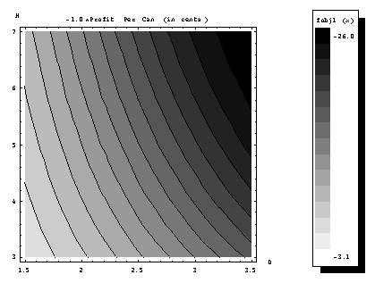
Figure 1.3.1: Profit-per-can contours for the
soft-drink-can example.
Next figure Figure 1.3.2 shows the contours of the profit per ounce for the
same example. Again, light regions correspond to low profit and dark regions to
high profit. This time the most
profitable soft-drink-can would appear to be around 2.5 inch diameter and 3
inches of height. In fact, the figure
hints that higher profits could possibly be realized if we could go to heights
below 3 inches. This is an indication
of the need to depict the constraints on the map in order to find the most
profitable can that satisfies the constraints, or the most profitable feasible
can.
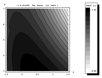
Figure 1.3.2:
Profit-per-ounce contours for the soft-drink-can example.
Figure 1.3.3 shows the constraints boundaries superimposed on the
profit contours. The constraint that
the diameter must range between 1.5 and 3.5 inches is accomodated by the
vertical boundaries of the map. The
minimum volume constraint (5 ounces) and the maximum volume constraint (15 ounces)
are two curves that are almost parallel to the cost contours. Finally, the aspect ratio constraint,
requiring that the height be at least twice the diameter is the straight line
connecting the two corners of the map.
The black line for each constraint depicts the boundary and was drawn
that way. For example, the boundary of the aspect-ratio constraint, g1,
is the line H = 2D drawn in the figure. Similarly, the minimum volume constraint, g2,
gives rise to the boundary 11.46 = H
D2, and the maximum volume constraint, g3,
gives rise to the boundary 34.38 = H D2. The convention is to draw hatch lines on the
side of the constraint that is infeasible.
In the figure, thick red lines indicate the infeasible side of the
constraint boundaries.
Figure 1.3.3:
Profit-per-can contours and constraints for soft-drink-can example.
The feasible domain in
Figure
1.1.1 is the pentagon with two slightly curved boundaries
in the upper left corner of the design space.
Actually, the top line H = 7 in. is not a boundary of the
feasible domain, as there is no constraint on a maximum value for H. However, the region for large values of H
is light, denoting low profit, so that there is no reason to extend the figure
in that direction.
The other four
boundaries correspond to four constraints.
Designs to the left of the D = 1.5 in. line have diameters which
are too small. Designs in the bottom
left corner of the design space do not have enough (5 ounces) volume. However, these two constraints are not
important, because they bound off regions of design space where profit is low
anyhow. Designs in the bottom right half
of the design space are too squat, they do not satisfy the aspect ratio constraint,
and designs in the top right corner are too big (more than 15 ounces).
The last two
constraints certainly limit the profit; they prevent access to the most
profitable (darkest regions) of the design space. It is clear from the figure
that the optimum design is found at the intersection of these two constraints,
that is for H = 2D and Vo = 15 ounces. We can find this intersection easily by
substituting H = 2D into the expression for the volume, and
setting it equal to 15 ounces to get
![]()
Solving this equation
we get D = 2.581 in., which corresponds to a height H = 5.162 in.
By using equations for the price-per-can, the cost of a can, and profit-per-can,
we find that the solution corresponds to selling a can for 33 cents, a cost of
17.23 cents, and a profit of 15.77 cents per can.
The design obtained
above maximizes the profit per can of the soft drink. However, this design does not correspond to the largest possible
profit per ounce. The constrained
design space for the profit per ounce of the soft drink is shown in the
following figure, Figure
1.3.4.
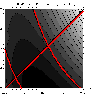
Figure 1.3.4:
Constrained design space for the profit-per-ounce of soft drink.
As opposed to the
previous solution, where two constraints were active, the darker region of the
design space, where the profit is the largest is, in the middle lower section
of the design space an is limited by only the aspect ratio constraint. In fact, the contour line bounding the
darkest section of the design space almost touches the aspect ration
constraint, indicating the possible location of the solution. Hence, in this case only the aspect ratio
constraint is active, H = 2D.
Substituting this into the equation for profit-per-ounce,
we get
![]() .
.
Now, we have a cost function with one variable. By taking the derivative of this function with respect to the can diameter and equating zero, we can find the solution to be D = 2.036 in., which corresponds to a height H = 4.072 in.
1.4.
Exercises 
1. A simply supported beam, 40 feet long, need to carry a uniformly distributed load of w = 1500 lb/ft. You would like to design a minimum weight beam with rectangular cross section (with b denoting the width and h the height of the cross section). Consider two failure modes, one in shear, and one bending. The maximum shear stress in the beam is
![]() ,
,
where A = b h is the cross-sectional area, and L=40 ft is the length. The maximum bending stress is
![]() .
.
You can choose to make the beam from steel, aluminum, or wood. The allowable shear stresses are 55,000 psi, 32,000 psi, and 1,000 psi, respectively. The allowable bending stresses are 100,000 psi, 60,000 psi, and 5,000 psi, respectively. The densities of the three materials are 0.28 lb/in3, 0.1 lb/in3, and 0.016 lb/in3. Additionally, we will run into problems of stability if the aspect ratio of the cross section is too high. Consequently, we do not permit the ratio between b and h to be larger than 5 or smaller than 0.2.
(a) Formulate the problem of designing the lightest weight steel beam in standard format, and using normalized constraints.
(b) Formulate the problem of designing the lightest weight beam using any of the three materials as a single optimization problem.
Hint: You can define three zero/one design variables that indicate whether or not you use any of the three candidate material, xs = 1 if you use steel and xs = 0 if you do not. Similarly, xa = 1 if you use aluminum, and xa = 0 if you do not, and for xw. Then the density of the material you use may be written as
r = 0.28 xs + 0.1 xa + 0.016 xw ,
with similar expressions for the allowable shear stress and bending stresses. You will need a constraint that will ensure that you use only a single material (that is that only one of the three variable can be equal to one), and this can be written as a simple equality constraint in terms of xs, xa, and xw.
2.
Solve graphically the beam design problem of Exercise 1. For each material, draw a map of weight
contours with the boundaries of the feasible domain superimposed, and each
constraint clearly labeled.
1.5.
References 
Barnett, R.L., “Minimum Weight Design of
Beams for Deflection," J. EM
Division, ASCE,
Vol. EM1, 1961, pp. 75-95.
Braibant,
V., Fleury, C., and Beckers, P., “Shape Optimal Design: An Approach Matching
C.A.D. and Optimization Concepts," Report SA-109, Aerospace Laboratory of
the University of Liege, Belgium, 1983.
Fox, C., An Introduction to the
Calculus of Variations, Dover Publications, 1987.
Prasad, B, and Haftka, R. T., “Optimal
Structural Design with Plate Finite Elements," ASCE J. Structural Division,
105, pp. 2367-2382, 1979.